Understanding Databricks Query Performance: A Practical Guide to Query Profile Analysis

Author: Abhishek Gautam

22 September, 2026

Introduction

When a SQL query takes longer than expected, execution time is usually the first thing we notice. But knowing that a query took 30 seconds or three minutes does not tell us why it was slow. The query may have scanned too much data, moved data between partitions, created a large intermediate result during a join, or simply required more memory than expected.

Databricks Query Profile helps us look beyond the final execution time and understand what actually happened while the query was running. It provides a visual execution plan along with metrics such as time spent, rows processed, memory usage, and data read. This makes it easier to identify performance bottlenecks and understand how data moved through the query.

Start With the Overall Query

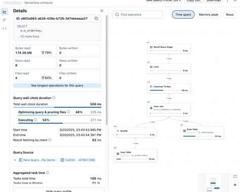
Before going deep into individual operators, I like to start with the overall query metrics. The first thing to understand is where the query spent its time. A query’s total duration can include the time Databricks spends preparing and optimizing the query, executing it, and returning the results. If most of the duration is spent during execution, the next step is usually to investigate the operators and the movement of data through the plan. If a significant amount of time is spent before execution begins, then query complexity, planning, metadata processing, or file pruning may deserve more attention.

I also look at the number of rows and bytes read, the number of files accessed, whether files were pruned, how much data came from cache, whether anything spilled to disk, and how many rows were eventually returned. These metrics provide useful context before looking at individual operators. A query returning only a few rows is not necessarily a small query. It may have read and processed a large amount of data before producing those few rows.

For example, if a query returns 12 rows but reads hundreds of files or millions of records to produce them, the small result set does not tell us how much work occurred behind the scenes. Looking at the overall metrics first gives us a better idea of what questions we should ask when we start exploring the execution plan.

Follow the Data Through the Query Plan

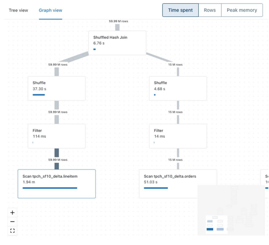
Once I understand the overall query, I start following the data through the execution plan. This is one of the most useful ways to approach Query Profile because it prevents us from focusing only on whichever operator happens to look the most expensive.

Consider a query that initially reads 120 million rows. An early filter reduces that data to 8 million rows before it reaches a join. The join produces 9 million rows, which are then aggregated down to 25,000 rows before the final 400 rows are returned. In this situation, most of the unnecessary data is removed early, which means the joins and aggregations downstream have much less data to process.

Now imagine the same 120 million rows moving through several joins before eventually being reduced to 8 million rows by a filter. Even if both queries produce the same final result, the second execution path may require substantially more intermediate processing. This is why one of the questions I keep asking while reading a query plan is simple: where did the amount of data suddenly increase or decrease?

Understanding Scans and Joins

A scan represents Databricks reading data from a source table. When looking at scans, I usually check the number of rows, files, and bytes being read and whether file pruning is occurring. If a query reads a large number of files but very little data is being eliminated through pruning, there may be an opportunity to reduce unnecessary reads.

Joins need a slightly different approach. The number of joins alone does not tell us whether a query is inefficient. A query with many joins can still perform well. What matters more is the join strategy, the amount of data entering the join, and how many rows come out of it. If a join receives one million rows but produces 15 million, that change deserves more attention than the join count itself.

What Is a Shuffle?

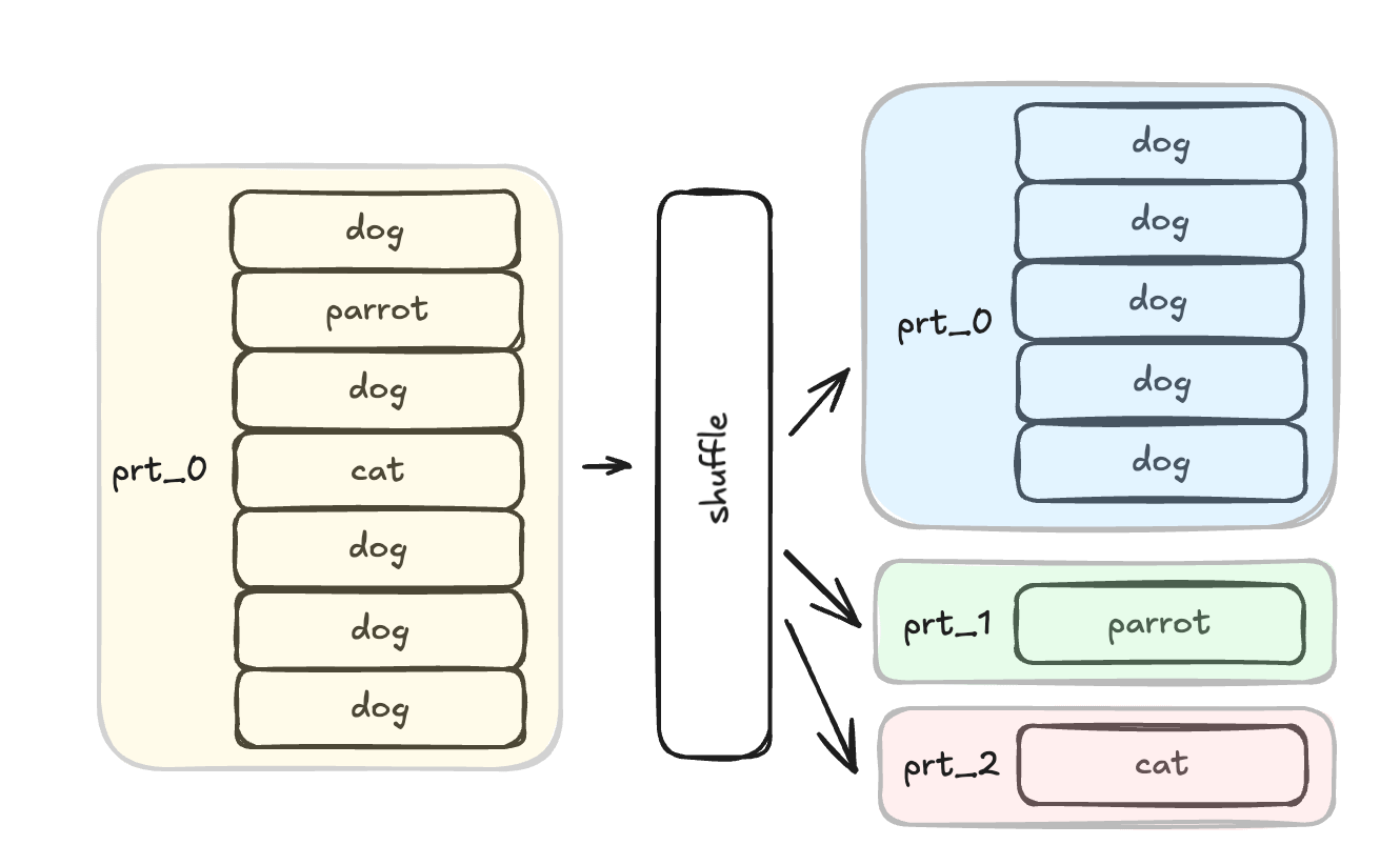
Shuffle is one of the most important concepts when analyzing Spark workloads. It happens when Spark needs to redistribute data across partitions so that related records can be processed together. This commonly happens during joins, aggregations, grouping, and sorting. Because data may need to move between executors, shuffle can consume network, memory, and execution resources. Databricks specifically identifies shuffle as a potentially expensive operation because of this data movement.

A shuffle does not automatically mean there is a performance problem. Instead, I look at how much data is being shuffled, how much time the operation requires, and how much memory it consumes. If shuffle accounts for a significant portion of execution time or peak memory, it becomes an area worth investigating.

Memory Usage and Spill

The Memory peak view helps identify which operators required the most memory during execution. Shuffles, joins, sorts, and aggregations can all require significant working memory, particularly when large intermediate datasets are involved.

High memory usage, however, does not necessarily mean that the query had a memory problem. The more important metric is whether data spilled to disk. Spill can occur when an operation cannot keep all of the intermediate data it needs in available execution memory. Some of that data then has to be temporarily written to disk, which can slow the query.

For example, a query may show that shuffle operators account for most of the peak-memory footprint while still reporting zero bytes spilled to disk. In that case, shuffle was memory-intensive, but the available memory was sufficient. This distinction is important because increasing compute simply because an operator has high memory usage may not address the real issue.

Find the Cause, Not Just the Symptom

One of the biggest lessons from Query Profile analysis is that the most expensive operator is not always where the problem started. An aggregation may appear slow because an earlier join created a very large intermediate dataset. A shuffle may require significant memory because too many rows reached it. A join may be expensive because filtering happened later than expected.

For this reason, when I identify an expensive operator, I usually trace backward through the execution plan. I look at what fed data into that operator, where the row count changed, and whether unnecessary work was introduced earlier. This makes it easier to distinguish the actual cause of a performance issue from the place where its impact eventually became visible.

A Repeatable Approach

A practical Query Profile analysis can follow a simple pattern. Start with the overall duration and the amount of data processed. Then use the Time spent view to identify expensive operations and the Rows view to understand how data volume changes through the plan. Review scans to understand how much data was read, and inspect joins and shuffles for row growth and data movement. Finally, use Memory peak together with spill metrics to determine whether memory actually became a constraint.

When optimizing a query, it is also useful to compare the Query Profile before and after the change. A faster execution time is useful, but the profile can explain why the query became faster. Perhaps fewer files were scanned, filtering occurred earlier, shuffle was reduced, or a large intermediate result was eliminated.

Conclusion

Query Profile analysis is less about finding a single “bad” operator and more about understanding how data moves through a query. The most useful questions are often simple: How much data did we read? Where did the number of rows change? Where did data need to move? Which operations required the most time or memory? Did anything spill to disk?

Following these questions through the execution plan makes it much easier to understand why a query behaves the way it does and where an optimization can have the greatest impact.